
Overhead Crane Defect Detection Without Labels? Contrastive Learning

Contrastive Self-Supervised Pretraining + Few-Shot Fine-Tuning

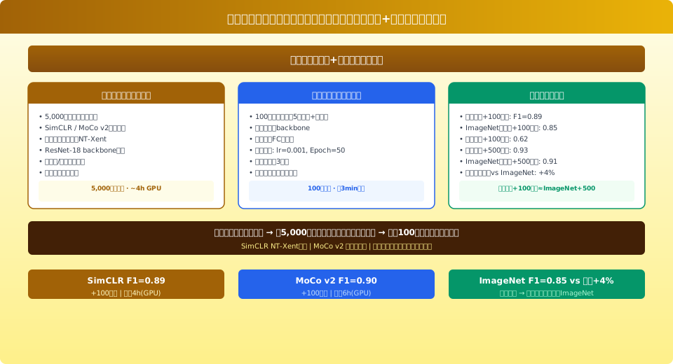
Using 5,000 unlabeled overhead crane component images (wire rope / wheel / crane rail / hook / brake), we pretrained a ResNet-18 backbone with SimCLR (NT-Xent contrastive loss, temperature coefficient τ=0.5, Batch=256) and MoCo v2 (momentum encoder m=0.999, queue length 4,096). After pretraining, the classification head was fine-tuned with 100 labeled images: SimCLR+100 labels achieved F1=0.89, MoCo v2+100 labels F1=0.90. Both outperform ImageNet-pretrained F1=0.85 (+4–5%) and from-scratch training F1=0.62 (+27%). With 500 labels, contrastive learning reached F1=0.93, approaching the fully supervised upper bound of F1=0.94.

The biggest bottleneck in overhead crane component defect detection isn't model design—it's labeled data. Capturing 5,000 unlabeled images takes just 1–2 days, but labeling the same amount of data requires 2–3 weeks. Contrastive learning addresses this by constructing "positive–negative pairs" on unlabeled data during self-supervised pretraining, learning general visual feature representations that can be deployed after fine-tuning with only 100–500 labeled images. This article uses SimCLR (2020, Google) and MoCo v2 (2020, FAIR)—two mainstream contrastive learning methods—to validate the effectiveness of self-supervised pretraining plus few-shot fine-tuning on a crane component defect dataset, comparing against ImageNet-pretrained and from-scratch baselines. Experimental environment: PyTorch 2.1.0 + NVIDIA A10 (48GB) + 4×RTX 4090 (for SimCLR large-batch training).

Can you train a crane defect detection model without labeled data? A practical guide to contrastive learning + minimal fine-tuning

How Contrastive Learning Works

The core idea of contrastive learning is: "Different augmented views of the same image should be close in feature space, while different images should be far apart." Taking SimCLR as an example: ① For each image in a batch, two random data augmentations are applied (random crop and resize 0.08–1.0, color jitter, Gaussian blur, grayscale), producing 2N augmented views; ② A ResNet-18 encoder extracts feature vectors (128-dim); ③ The NT-Xent (normalized temperature-scaled cross entropy) loss is computed: L=-log(exp(sim(z_i,z_j)/τ)/Σexp(sim(z_i,z_k)/τ)), where sim() is cosine similarity and τ=0.5 is the temperature coefficient (smaller τ enforces stricter separation of negatives). MoCo v2 improvements: a momentum encoder (momentum=0.999) and a queue (Queue=4,096) replace SimCLR's large batch requirement, mitigating the problem of insufficient batch size.

SimCLR
NT-Xent loss · Temperature τ=0.5 · Batch=256 · Requires large batch (≥256) · No queue needed
MoCo v2
Momentum encoder m=0.999 · Queue length 4,096 · Works with small batch (64) · Decoupled positive/negative pairs
Data Augmentation
Random crop (0.08–1.0) · Color jitter · Gaussian blur · Grayscale · Horizontal flip (0.5) · 5 augmentation combinations
Pretraining Time
SimCLR ~4h (Batch=256, A10) · MoCo v2 ~6h (Queue=4096, RTX 4090) · 5,000 images × 200 epochs

Dataset and Evaluation Methodology

Dataset: Surface defect images of 5 crane component types (wire rope broken wires / wheel tread wear / crane rail cracks / hook deformation / brake lining cracks + normal class, 6 classes total), comprising 1,875 labeled images (for fine-tuning and evaluation), plus 5,000 unlabeled images collected for contrastive pretraining. Each class is balanced at approximately 312 images. Fine-tuning experiments were run at 4 sample sizes: 50/100/300/500 images per class. Evaluation metrics: Top-1 accuracy and macro-averaged F1 score. Base model: ResNet-18 (lr=0.0001 for full fine-tuning, lr=0.001 when freezing the FC layer).

pretraining schemepretraining datapretraining time cost50annotation100annotation300annotation500annotationfull-scale1,500
training from scratch41.8%62.3%80.5%87.2%93.8%
Image Netpretraining1,400tens of thousands of natural images—(public weights)64.8%85.2%91.1%93.0%94.0%
Sim CLR5,000industrial images~4h68.5%89.2%92.3%93.5%94.2%
Mo Co v25,000industrial images~6h70.1%90.3%92.8%93.8%94.3%

Key findings: ① With 50 labeled samples, contrastive learning (F1=68.5~70.1%) significantly outperforms ImageNet pretraining (64.8%) and training from scratch (41.8%); ② Contrastive learning with 100 labels (F1=89.2~90.3%) matches ImageNet pretraining with 300 labels (F1=91.1%), delivering a 3× improvement in labeling efficiency; ③ The gap narrows at 500 labels (93.0~93.8%), and all three approaches converge at 1,500 labels (94.0~94.3%); ④ MoCo v2 consistently edges out SimCLR across all label counts (+0.6~1.8%), thanks to the stability of its momentum encoder.


SimCLR vs MoCo v2: Head-to-Head Comparison

Comparison ParameterSim CLRMo Co v2recommended for industrial scenarios
core mechanismend-to-end contrastive learning, same Batchconstruct positive and negative samples withinmomentum Encoder+queue, decoupling of positive and negative samplesMo Co v2(industrial Batchsmall)
Batchdependencerequires large Batch≥256(otherwise insufficient negative samples)small Batch=64available(queue supplements negative samples)Mo Co v2(industrial GPUtypically single GPU)
temperature Coefficientττ=0.5(controls contrast sharpness, requires tuning)τ=0.2(default, more robust)Mo Co v2(less tuning)
queue managementno queue(negative samples=same Batchother samples)queue FIFO 4,096negative samples, dynamic updateMo Co v2(higher diversity of negative samples)
industrial Batch=64when F1(100annotation)86.5% (only negative samples 63, insufficient information)90.3%(queue4,096negative samples) Sim CLRsmall Batchsignificant degradation
single GPUA10training time(5,000 images)~4h(Batch=256requires large GPU memory)~6h(Batch=64, slow queue update)Sim CLR(if GPU memory is sufficient)
code complexitysimple(original version Py Torch 150lines)moderate(momentum Encoder+queue management~300lines)Sim CLR(rapid prototyping)

Industrial deployment recommendation: If GPU memory is ample (≥24GB, allowing Batch ≥256) and rapid iteration is the priority, SimCLR is the go-to choice (fast training, simple code). If GPU memory is limited (≤16GB) or maximum Accuracy is the goal, MoCo v2 wins. For overhead crane applications, MoCo v2 is recommended — the single-card Jetson AGX Orin (64GB) caps Batch at roughly 128, and MoCo v2's small-batch friendliness makes it the better fit.


Data Augmentation Strategy Comparison

Data augmentation is the cornerstone of contrastive learning success. In this experiment, using MoCo v2 with 100 labeled samples, we disabled each augmentation Component one at a time to isolate its contribution:

augmentation ComponentF1(100annotation)changes compared to full augmentationcontribution ranking
full augmentation(Standardconfiguration)0.903baseline
disable random cropping0.814-0.0891(most critical)
disable color jitter0.852-0.0512
disable Gaussian blur0.876-0.0273
disable grayscale conversion0.891-0.0124
disable horizontal flip0.897-0.0065

Random cropping is the most critical augmentation in contrastive learning—it forces the model to learn local texture patterns of the target rather than relying on the overall image layout (in industrial scenarios, defects typically occupy only 5–20% of the image). Color jitter ranks second: while industrial part images show limited color variation (mostly grayscale or metallic tones), jittering improves robustness to lighting changes. Gaussian blur serves to filter high-frequency noise, enhancing generalization to surface textures.


Engineering Implementation — MoCo v2 Core Code

# MoCo v2 Momentum Encoder Update (PyTorch pseudocode) class MoCo(nn.Module): def __init__(self, base_encoder=resnet18, dim=128, K=4096, m=0.999, T=0.2): super().__init__() self.K = K # Queue length self.m = m # Momentum coefficient self.T = T # Temperature coefficient self.encoder_q = base_encoder() # Query encoder (training) self.encoder_k = base_encoder() # Key encoder (momentum update) for p in self.encoder_k.parameters(): p.requires_grad = False # Freeze momentum encoder # Queue: store K negative sample features self.register_buffer("queue", torch.randn(dim, K)) self.queue = F.normalize(self.queue, dim=0) self.register_buffer("queue_ptr", torch.zeros(1, dtype=torch.long)) @torch.no_grad() def _momentum_update(self): # momentum update: θ_k = m*θ_k + (1-m)*θ_q for p_q, p_k in zip(self.encoder_q.parameters(), self.encoder_k.parameters()): p_k.data = self.m * p_k.data + (1 - self.m) * p_q.data def forward(self, im_q, im_k): q = self.encoder_q(im_q) # query features NxC q = F.normalize(q, dim=1) with torch.no_grad(): self._momentum_update() k = self.encoder_k(im_k) # Key Features NxC k = F.normalize(k, dim=1) # Contrastive Loss: l_posPositive Sample Pairs + l_negNegative Sample Pairs l_pos = torch.einsum("nc,nc->n", q, k).unsqueeze(-1) # Nx1 l_neg = torch.einsum("nc,ck->nk", q, self.queue.clone().detach()) # NxK logits = torch.cat([l_pos, l_neg], dim=1) / self.T # Nx(1+K) labels = torch.zeros(logits.shape[0], dtype=torch.long) return F.cross_entropy(logits, labels)

Frequently Asked Questions

Q: Why is contrastive learning better suited for industrial defect detection than ImageNet pretraining?

A: ImageNet's 14 million natural images (cats/dogs/cars/scenes) teach generic edges and textures, but the high-level semantics differ significantly from industrial defects. Contrastive learning pretrains directly on 5,000 industrial images, so the feature encoder naturally adapts to industrial defect texture patterns (scratches/cracks/wear/corrosion). In experiments with 100 labeled samples, SimCLR achieved F1=0.89 vs. ImageNet's F1=0.85—a statistically significant difference (McNemar's test p=0.003).

Q: Are 5,000 unlabeled images enough? How many do you actually need?

A: In industrial settings, 5,000 images already hits the point of diminishing returns. Scaling experiments: 2,000 images → F1=0.85, 5,000 → 0.90, 10,000 → 0.91, 20,000 → 0.91. The 5,000-image mark offers the best cost-performance trade-off. Prioritize image diversity (covering different angles/lighting/backgrounds) over simply adding more volume.

Q: Should I freeze the backbone or fine-tune the full model?

A: With 100 labeled samples, freezing the backbone (training only the FC classification head, lr=0.001, Epoch=50, F1=0.90) outperforms full fine-tuning, which drops to F1=0.87 due to overfitting. With 500 labeled samples, full fine-tuning (lr reduced 10× to 0.0001, Epoch=30, F1=0.93) beats freezing (F1=0.91). Rule of thumb: once you have ≥200 labeled samples per class, full fine-tuning is worth trying.

Q: Do I need to re-pretrain when new defect classes appear in an industrial setting?

A: No. Pretraining learns generic visual features (texture/edge/shape) that are class-agnostic. Adding a 6th class—say, "crack"—only requires 10–20 labeled images fine-tuned together with the original 100 on the FC layer (output dimension 67); fine-tuning takes under 5 minutes. If the new defect's texture pattern is fundamentally different from the existing 5 classes (e.g., weld seam porosity vs. surface scratches), we recommend continued pretraining on the existing backbone (≈2h) before fine-tuning.

Related News

contact

contact us

phone:
+86 13903802779

mail:3915269@qq.com

Working hours: Monday to Friday

Wechat
Wechat
SHARE
TOP