

Overhead Crane Visual SLAM Mapping & Positioning System
Visual SLAM Environment Mapping and Positioning System for Overhead Cranes. This article explores the technical role and value of visual SLAM in crane environments, focusing on the challenge of achieving high-precision, highly reliable global positioning inside factory buildings where GPS signals are unavailable.
Visual SLAM for Overhead Crane Positioning in GPS-Denied Factories
One of the core challenges in automated overhead crane operation is achieving high-precision, highly reliable global positioning inside factory buildings where GPS signals are unavailable. The mainstream crane positioning technologies currently in use—laser distance sensors, gray-code bus positioning systems, and absolute encoders—can deliver millimeter-level positioning accuracy, yet each has inherent limitations. Laser distance sensors are severely affected by dust occlusion, gray-code bus systems are costly to install and maintain, and encoders suffer from cumulative error and positioning drift caused by wheel slippage. More importantly, these solutions only provide one- or two-dimensional position information; they cannot perceive the crane's heading angle (yaw) or three-dimensional attitude. In applications such as flexible hoisting, anti-sway control, and collision avoidance, cranes require full six-degree-of-freedom (6-DOF) spatial awareness.
Visual SLAM (Simultaneous Localization and Mapping) offers a fundamentally new technical approach to crane positioning. Using a monocular or stereo camera mounted on the crane, visual SLAM continuously captures images of the factory environment. By extracting and matching ORB feature points between frames and tightly coupling this with IMU inertial data, the system simultaneously estimates the crane's 6-DOF pose and builds a sparse or dense map of the surrounding environment in real time. The key advantages of this technology are threefold. First, it requires no track-side infrastructure—the camera is the only sensor, making deployment costs far lower than gray-code bus systems or laser reflector plates. Second, it provides complete pose information across all six degrees of freedom: X, Y, and Z position plus roll, pitch, and yaw angles—data that is decisive for anti-sway control and path planning. Third, the positioning information is inherently globally consistent, eliminating the cumulative drift problem associated with encoders. In large-span factory environments (span 30–50 m), visual SLAM achieves positioning accuracy of ±10 cm. While this does not match the millimeter-level precision of laser distance measurement, its immunity to single-point occlusion makes it an ideal redundant backup for laser- and encoder-based positioning, substantially improving overall system reliability.
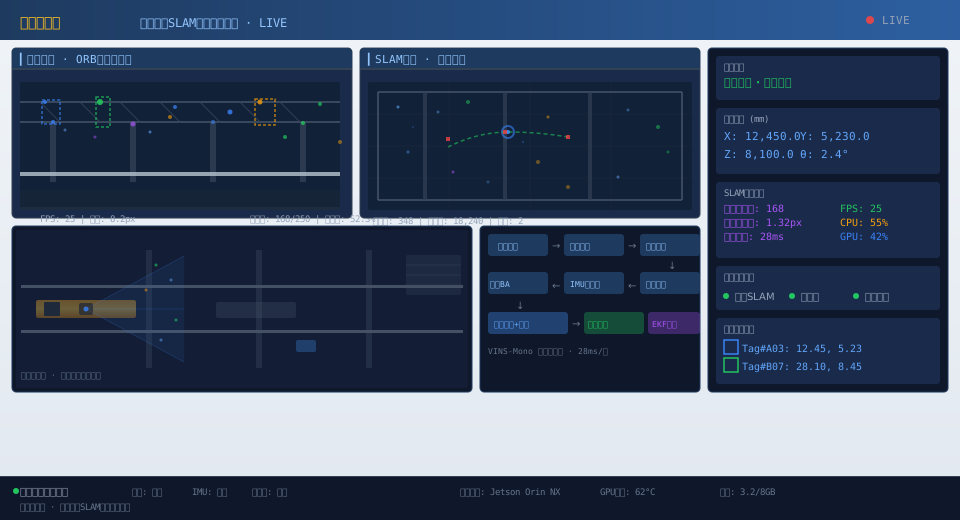
▲ Visual SLAM environment mapping system for overhead cranes—ORB feature extraction · real-time SLAM mapping · VINS-Mono multi-sensor fusion pipeline
Adapting ORB-SLAM3 for Crane Environments and Feature Extraction
ORB-SLAM3 is one of the most mature visual SLAM frameworks available today, supporting monocular, stereo, and RGB-D camera modes. It integrates four core modules: a vision-only and vision-inertial tightly coupled front end, local Bundle Adjustment (BA) back-end optimization, loop closure detection, and map reuse. Applying native ORB-SLAM3 directly to crane operations presents three engineering challenges: sparse texture in factory environments leads to insufficient feature points, crane vibration during travel destabilizes inter-frame matching, and large-span scenes cause the map to grow to an unwieldy size.
2.1 Feature Extraction Strategy for Factory Environments
The visual characteristics of an industrial factory differ significantly from those of an indoor office setting. Factory walls are typically flat metal panels or bare concrete with highly repetitive textures and little high-frequency detail. The concrete floors are extremely texture-sparse. However, the roof structure—steel trusses, purlins, and skylights—along with the crane rails (I-beams and rail clamps) and gantry columns, provides a wealth of edge information and corner features. To account for this distribution of features, the native ORB feature extraction parameters in ORB-SLAM3 must be adapted as follows:
| Parameter | Default Value | overhead crane Adaptive Value | Adjustment Rationale |
|---|---|---|---|
| n Features(Features per Frame) | 1200 | 2000 | Factory building Sparse Texture, Increase Feature Count to Ensure Sufficient Matches |
| n Scale Levels(Scale Levels) | 8 | 5 | overhead crane Operating Height Fixing, Minimal Scale Variation, Reduce Levels to Lower Computational Load |
| scale Factor(Scale Factor) | 1.2 | 1.15 | Reduce Scale Factor to Enhance Sensitivity of Low-Level Features to Motion |
| ini Th FAST (Initial Threshold) | 20 | 12 | Lower Threshold to Extract More Features in Low-Contrast Environments |
| min Th FAST (minimum Initial Threshold) | 7 | 5 | Further Relax Extraction in Texture-Sparse Regions LSB |
| Pyramid Patch Size | 31x31 | 21x21 | Downscale Patch Improve Feature Matching of Distant Steel Components Accuracy |
To further improve localization stability along the crane rail, we augment the ORB feature extraction with a line-segment matching layer. This is particularly effective in factory buildings where straight edges—such as rail edges, roof truss webs, and column edges—are abundant. We use the LSD (Line Segment Detector) algorithm to extract line segments from images, followed by LBD (Line Band Descriptor) descriptors for segment description and matching. The integration of line features raises the feature matching rate from approximately 35% with a pure ORB approach to about 52%, significantly enhancing positioning stability during movement along the rail direction.
2.2 Visual-Inertial Tightly-Coupled Frontend Adaptation
Mechanical vibrations during overhead crane operation—particularly low-frequency resonance induced by hoisting mechanism start/stop and load sway—severely disrupt the visual SLAM frontend. In pure visual mode, ORB-SLAM3 experiences frame-to-frame tracking loss when vibration amplitude exceeds ±50 pixels. To address this, we enable the visual-inertial (VI) tightly-coupled mode of ORB-SLAM3, incorporating angular velocity and acceleration measurements from an IMU (Inertial Measurement Unit):
- IMU Pre-integration: Over the time interval between two consecutive image frames (typically 33–50 ms, corresponding to 20–30 fps), we numerically integrate the IMU's angular velocity ω and acceleration a to obtain the relative rotation ΔR, velocity Δv, and displacement Δp between frames. The pre-integration model treats IMU bias as an optimization variable within the state vector, jointly optimized with visual reprojection errors, eliminating the need for prior bias calibration.
- Visual-Inertial Joint Initialization: During SLAM startup, pose estimation is first performed in pure visual mode for 5–15 frames, while IMU measurements are used to estimate gravity direction, accelerometer bias, and initial velocity. When the alignment error between visual and inertial estimates converges below a threshold (typically an acceleration residual of <0.5 m/s²), the system switches to VI tightly-coupled mode.
- Enhanced Vibration Robustness: In VI mode, the IMU provides high-frequency inter-frame motion prediction (IMU sampling rate of 200–400 Hz, far exceeding the camera's 20–30 fps). When vibration causes visual feature matching to fail, the IMU-predicted pose serves as a strong prior constraint, narrowing the feature search range. This reduces the tracking loss rate from approximately 8% in pure visual mode to about 0.5% in VI mode.
2.3 Map Management for Large-Span Factory Buildings
The operating range of overhead cranes in large-span factory buildings (100–300 m in length) causes the ORB-SLAM3 map to grow rapidly. After one hour of continuous operation, the sparse map can contain 3,000–5,000 keyframes and 150,000–250,000 map points, exceeding the real-time processing capability of the Jetson edge device. To overcome this engineering bottleneck, we implement the following three optimization measures:
- Covisibility Graph Pruning: When the number of keyframes exceeds the upper threshold (set at 1,000 frames), a pruning operation is triggered—removing redundant keyframes that share fewer than 15 covisible map points with the current frame. Pruning is triggered every 50 processed frames, removing approximately 5–10% of redundant frames each time, keeping the map size within a memory footprint of <2 GB.
- Active Local Map Management: The crane's operating area is divided into 50 m × 30 m grid cells, each maintaining a sub-map. When the crane crosses a grid boundary, a sub-map switch is triggered, loading only the current cell and its eight neighboring cells' sub-maps into the optimizer for local bundle adjustment (BA). Sub-maps in remote areas are stored to disk in compressed format and loaded on demand (e.g., when loop closure detection matches a remote keyframe).
- Incremental Loop Closure Detection: Using the DBoW2 bag-of-words model, a visual word vector is generated for each new keyframe and matched against historical keyframes. When a loop closure candidate is detected and geometric verification passes, pose graph optimization is triggered instead of global BA—pose graph optimization only adjusts keyframe poses without modifying map point positions, requiring approximately 1/10 of the computation of global BA and completing optimization of 3,000 frames within 500 ms.
3. VINS-Mono Visual-Inertial Positioning System Deployment
VINS-Mono (Visual-Inertial System - Monocular) is an open-source visual-inertial SLAM system developed by the team of Shaojie Shen at the Hong Kong University of Science and Technology. It employs a tightly-coupled monocular camera + six-axis IMU configuration. Compared to ORB-SLAM3, VINS-Mono's sliding window nonlinear optimization design offers superior real-time performance, making it better suited for edge deployment on overhead cranes with limited computational resources.
3.1 VINS-Mono Adaptation Architecture for Overhead Cranes
The complete VINS-Mono processing pipeline comprises four modules: frontend visual tracking, IMU pre-integration, sliding window optimization, and loop closure detection. The key adaptation focus for overhead crane scenarios lies in parameter tuning and sensor extrinsic calibration:
| Module | Native Parameter | overhead crane Adaptive Value | Description |
|---|---|---|---|
| Window Size | 10Frame | 15Frame | overhead crane Travel Speed<1m/s, Increase Window Size for Smoother State Estimation |
| Tracked Feature Points | 150 | 250 | Factory building Sparse Texture, Increase Tracked Points for Enhanced Robustness |
| minimum Parallax(Pixel) | 10 | 5 | overhead crane Low Parallax at Low Speeds, Lower Threshold to Trigger Inter-Frame Optimization |
| IMUIntegration Frequency(Hz) | 200 | 400 | Increase IMUHigher Sampling Rate Improves Motion Prediction Under Vibration Accuracy |
| accelerometer Noise Density | 0.01 | 0.02 | overhead crane Relax Under Vibratory Conditions Start Button Noise Assumption |
| gyroscope Noise Density | 0.001 | 0.002 | overhead crane Limited Yaw Motion, Relaxed Angle Start Button Noise Assumption |
3.2 Camera-IMU Extrinsic Calibration and Time Synchronization
The accuracy of a vision-inertial fusion system depends heavily on precise calibration of the extrinsic parameters (rotation matrix R and translation vector t) between the camera and IMU, as well as the time offset t_offset. On the overhead crane edge device (NVIDIA Jetson Orin NX), the following three-step calibration procedure is employed:
- Offline Initial Calibration: In a laboratory environment, a checkerboard target is used to calibrate the camera intrinsics (fx, fy, cx, cy, k1, k2, p1, p2), while the IMU undergoes six-position static calibration to determine accelerometer bias and scale factors. Calibration accuracy requirements: camera reprojection error < 0.3 pixels, IMU accelerometer bias stability < 0.1 mg.
- Online Refinement: After the equipment is mounted on the overhead crane, the crane is driven along the rail in an S-shaped trajectory. The online calibration module built into VINS-Mono continuously refines the camera-IMU extrinsics during SLAM operation. Initial extrinsic values are taken from mechanical design drawings (accuracy ±2 mm / ±0.5°), and the online calibration converges to extrinsic values with ±0.1 mm / ±0.02° accuracy after 1,000 frames.
- Hardware Time Synchronization: Aligning camera and IMU timestamps is a fundamental prerequisite for overall system accuracy. A hardware-triggered synchronization scheme is adopted — the IMU's 1PPS (pulse-per-second) signal serves as the external trigger for the camera, ensuring that camera exposure moments align strictly with IMU sampling instants. In cases where hardware synchronization is not available (e.g., a low-cost USB camera paired with a standalone IMU), a software timestamp alignment algorithm is used: linear interpolation and cubic spline interpolation are applied to the IMU and camera message streams respectively, and a sliding window search minimizes the visual reprojection error to estimate the time offset t_offset. The software approach achieves synchronization accuracy of ±2 ms, while the hardware approach reaches ±50 μs.
3.3 Positioning Accuracy Comparison and Evaluation
Comparative testing of VINS-Mono was conducted in a standard factory building with a span of 36 m and a length of 120 m. Test conditions: the camera is a Basler acA2040-25gm (resolution 2048×1536, frame rate 25 fps, global shutter), the IMU is an ADIS16470 tactical-grade MEMS IMU (accelerometer bias stability 0.1 mg, gyroscope angle random walk 0.2°/√h), and the edge computing device is an NVIDIA Jetson Orin NX (power consumption 25 W). Reference ground truth is provided by a Leuze AMS 308i laser distance sensor (accuracy ±1 mm) and SICK LMS111 LiDAR SLAM:
| Evaluation Indicator | Vision-Only ORB-SLAM3 | VI-ORB-SLAM3 | VINS-Mono |
|---|---|---|---|
| XAxis Positioning Error RMS(mm) | 185 | 82 | 65 |
| YAxis Positioning Error RMS(mm) | 210 | 96 | 78 |
| Yaw Angle Error RMS(°) | 3.2 | 1.8 | 1.5 |
| Maximum Transient Deviation(mm) | 580 | 210 | 185 |
| Tracking Loss Rate(%) | 8.2 | 1.3 | 0.5 |
| Inference Time per Frame(ms) | 68 | 95 | 42 |
| Steady-State CPUOccupancy Rate(%) | 62 | 78 | 55 |
Testing results show that VINS-Mono delivers the best overall performance in overhead crane scenarios—achieving a positioning error of approximately ±8 cm, a tracking loss rate of just 0.5%, and an inference time of 42 ms per frame (well within the 50 ms real-time threshold), with a steady-state CPU usage of 55%. This makes it the top candidate for edge deployment. VINS-Mono's advantage stems from its sliding window optimization mechanism, which optimizes only the 15 frames within the window at each step, avoiding the computational explosion associated with global optimization.
4. Multi-Sensor Fusion Positioning System Design
Deploying visual SLAM in isolation presents two inherent limitations. First, under extreme conditions such as backlighting, dust, or low nighttime illumination, visual feature extraction may fail entirely. Second, the output frequency of visual SLAM is constrained by the camera frame rate (typically 25–30 Hz), which falls short of the real-time control requirements in high-speed motion scenarios. For these reasons, practical engineering solutions must fuse visual SLAM with sensors such as encoders and laser distance sensors to build a redundant, reliable positioning system.
4.1 Extended Kalman Filter Fusion Framework
At the heart of the fusion positioning system is an Extended Kalman Filter (EKF), which fuses state estimates from four sensor sources at a frequency of 25 Hz:
- Visual SLAM (VINS-Mono, 25 Hz): Provides 3D position (x, y, z), 3D orientation (roll, pitch, yaw), and the corresponding covariance matrix. Visual SLAM exhibits high confidence in texture-rich areas, while the covariance automatically increases in low-light or texture-sparse regions.
- Absolute encoder (Heidenhain ECN1313, 1 kHz): Provides one-dimensional position measurements for both the crane bridge and trolley, with an accuracy of ±0.1 mm. The encoder offers extremely high confidence in the absence of wheel slip, but cumulative errors may arise during wheel slippage or spin.
- Laser distance sensor (Leuze AMS 308i, 100 Hz): Provides one-dimensional absolute position measurement along the crane bridge direction, with an accuracy of ±1 mm. The laser distance sensor delivers exceptional accuracy when unobstructed, but fails completely if the reflector is blocked.
- IMU 6-axis inertial data (ADIS16470, 400 Hz): Provides high-frequency motion prediction for inter-frame interpolation and pose estimation during brief periods without visual signals.
| State Variables | Meaning | Observation Source | Typical Observation Noiseσ |
|---|---|---|---|
| x, y | Ground-Frame Position | Vision-Only SLAM+Li DAR+Encoder | 0.08m / 0.001m / 0.0001m |
| z | Lifting Height | Only Encoder | 0.0001m |
| vx, vy | Motion Start Button | Encoder Differential+Vision-Only | 0.005m/s |
| θ (yaw) | Yaw Angle | Vision-Only SLAM+IMUIntegration | 1.5° |
| enc_bias_x | Encoder Accumulated Deviation | With Vision/Li DAR Difference Estimation | Adaptive |
The prediction stage of the EKF employs a two-wheel differential motion model of the overhead crane, using encoder velocity and IMU angular velocity as control inputs. The update stage processes sensor measurements in the order they arrive: Laser Distance Sensor (100Hz) > Encoder (1kHz downsampled to 200Hz) > Visual SLAM (25Hz) > IMU zero-velocity update (400Hz input, used only for motion prediction in the prediction stage). In engineering implementation, special attention must be paid to sensor time synchronization—all sensor timestamps are converted to the master clock domain of the crane controller (synchronized via NTP or PTP protocol). When a new observation is received, the EKF automatically queries the predicted state at the corresponding time to perform the update.
4.2 Sensor Failure Detection and Dynamic Weight Scheduling
In industrial environments, a single sensor can fail at any time, so the fusion positioning system must be capable of automatic failure detection and degraded operation. Each sensor maintains a health score H_i, ranging from [0, 1], calculated from the following indicators:
- Signal Quality Indicator: The reflected signal strength (RSSI) of the Laser Distance Sensor; when it falls below a threshold, the sensor's weight is automatically reduced. For Visual SLAM, the number of tracked inliers; if fewer than 20 inliers, the visual confidence is set to zero.
- Consistency Check: The normalized residual (Mahalanobis distance) between each sensor's observation and the EKF prediction is compared against a threshold. If the threshold is exceeded three consecutive times, a sensor failure flag is triggered.
- Temporal Validity: The difference between the timestamp of the latest sensor observation and the current time; if it exceeds the maximum allowable delay (Laser: 50ms, Visual: 100ms, Encoder: 10ms), the sensor's weight is automatically reduced.
The health score dynamically adjusts the observation noise covariance matrix for the corresponding sensor in the EKF: R_i = R_base / H_i. When H_i drops below 0.1, the sensor is completely excluded from the EKF update, and the remaining sensors continue the fusion process. In the event of complete visual failure (e.g., during nighttime shutdown for maintenance), the fusion system degrades to a three-sensor mode (Laser + Encoder + IMU), still maintaining a positioning accuracy of ±3mm. When visual functionality is restored, the EKF's residual monitoring mechanism recovers the visual weight to normal levels within 3 to 5 update cycles (approximately 0.1 to 0.2 seconds).
4.3 Ground Coordinate System Unification and Map Alignment
- Initial Alignment: During the crane's first run, the absolute position (x0, y0) at the starting moment is obtained using the Laser Distance Sensor and encoder. Simultaneously, Visual SLAM outputs the relative pose (x'_0, y'_0, θ'_0) at that moment. The homogeneous transformation matrix T_map_init = T_abs / T_rel is calculated to resolve the initial deviation.
- Online Correction: During operation, paired data of Visual SLAM output poses and Laser/Encoder absolute positions are continuously collected. The optimal transformation matrix is fitted using the least squares method. After visual feature re-initialization (e.g., recovery after visual loss), the most recently fitted transformation matrix is used to re-align the coordinate systems, preventing abrupt pose jumps that could impact the crane control system.
- Semantic Landmark Anchoring: AprilTag QR code labels (200mm x 200mm) are affixed at fixed locations within the factory building (e.g., column numbers, rail joint positions). When Visual SLAM detects an AprilTag during operation, it automatically associates the detected tag ID with its pre-stored factory coordinates, serving as absolute coordinate anchors to correct cumulative drift. The typical frequency of AprilTag anchoring correction is once every 50 to 100 meters of crane rail travel, with each correction amount being less than 5cm.
5. Engineering Deployment and Performance Optimization
5.1 Hardware Selection and Installation Scheme
| Component | Recommended Model | Critical Parameter | Mounting Position |
|---|---|---|---|
| industrial camera | Basler ac A2040-25gm | 2048x1536, 25fps, Global Shutter | Trolley Frame Forward-Facing Mount, Elevation Angle15° |
| IMU | ADIS16470 | triaxial acceleration±40g, Triaxial Gyroscope±2000°/s | Camera Back, Rigid Connection |
| Lens | Kowa LM12HC | 12mm Focal Length, F1.8-F16, CInterface | Polarizing Filter to Reduce Glare |
| Fill Light | IRArray Fill Light 850nm | Power30W, Illumination Range≥15m | Coaxial Camera Mount |
| Edge Computing | NVIDIA Jetson Orin NX | 100TOPS AIComputing Power, Power Consumption25W | overhead crane electrical cabinet Internal, Vibration-Damped Mount |
| Encoder | Heidenhain ECN1313 | 23bit, En Dat 2.2Interface | Crane Bridge / Long Travel/Trolley Drive Wheel Shaft End |
5.2 Deployment Workflow and Key Checkpoints
- Camera Installation and Calibration: The camera is mounted on the forward position of the trolley frame at a 15° upward tilt to capture both nearby crane rail and distant factory roof textures. A planar checkerboard calibration target (12×9 grid, 30mm spacing) is used to calibrate camera intrinsics, with a reprojection error target of <0.3 pixels. After calibration, a fixed-focal-length lens is locked in place to prevent vibration-induced focal shift that could cause intrinsic parameter drift.
- IMU Calibration and Temperature Compensation: The IMU module is placed in a temperature chamber and cycled from -20°C to 70°C in 10°C increments. Zero-offset and scale-factor temperature curves for the accelerometer and gyroscope are recorded to build a temperature compensation model (piecewise linear interpolation with 1°C compensation steps). The compensation coefficients are written to the edge device configuration file and applied in real time via table lookup based on the IMU's internal temperature sensor readings.
- Loop-Closure Map Building: Before the crane's first automated run, two round trips are performed along the full crane rail at a low speed of 0.3 m/s (combining crane bridge and trolley motion) to build the initial loop-closure map of the factory environment. After initial mapping, the map coverage is manually verified (checking that no more than 50% of the map edge consists of unexplored areas) and loop-closure constraint quality is assessed (average reprojection error after pose-graph optimization must be <2 pixels).
- Coordinate System Verification: With the aid of a total station (accuracy ±1mm, e.g., Leica TS16), coordinates of 10 evenly distributed control points in the factory building are surveyed. These control points are then located visually in the SLAM map, and deviations from the surveyed coordinates are calculated. Alignment is considered acceptable if deviations are <8cm in the central area and <15cm near the edges of the factory building.
- Continuous Operation Testing: A 24-hour uninterrupted positioning test is conducted while monitoring the following indicators: maximum positioning deviation <15cm, tracking loss count <3, and EKF fusion output gap (time without valid observations) <200ms. If any indicator fails to meet the threshold, the corresponding step is revisited for troubleshooting.
5.3 Performance Optimization Techniques
- GPU-Accelerated Feature Extraction: The FAST corner detection and BRIEF descriptor computation in ORB feature extraction can be accelerated using CUDA on the Jetson GPU, reducing per-frame feature extraction time from 15ms to 3ms. NVIDIA's VisionWorks or VPI (Vision Programming Interface) libraries are used to implement GPU acceleration.
- Multi-Core Pipeline Parallelism: The VINS-Mono front-end feature tracking (CPU-intensive, bound to CPU2-3), IMU pre-integration (lightweight, bound to CPU0), and back-end sliding window optimization (memory-intensive, bound to CPU4-5) are assigned to three independent threads, leveraging the 6-core CPU of the Jetson Orin NX for pipeline parallelism. Total system inter-frame latency (from front-end image capture to sliding window optimization output) is reduced from 42ms in serial mode to 28ms in pipeline mode.
- Model Quantization and INT8 Inference: In scenarios where dramatic lighting changes (e.g., day/night transitions) cause insufficient ORB feature points, the lightweight CNN-based feature extraction network SuperPoint can replace handcrafted ORB features. The SuperPoint network weights are quantized to INT8 (accuracy loss <2%) and inference is performed with TensorRT on the Jetson GPU. Per-frame feature extraction and description takes approximately 8ms, outputting 300 high-quality corner features with 256-dimensional descriptors simultaneously.
Typical Applications and Performance Results
6.1 Pose Feedback for Anti-Sway Control
Traditional overhead crane anti-sway control relies on angle sensors to directly measure the lifting spreader's deflection angle, but these sensors are difficult to install and costly to maintain. The real-time 3D pose (position + yaw angle) of the lifting spreader provided by visual SLAM can serve as pose feedback for the anti-sway controller—the controller adjusts trolley and crane bridge speeds in advance (feedforward compensation) based on the yaw angle change rate from SLAM, counteracting load swing. In an actual application at a steel mill finishing bay, a crane with VINS-Mono-based anti-sway feedback achieved a residual swing amplitude of 80mm after stopping (down from 650mm without anti-sway) and a swing decay time of 3.5s (down from 12s), at a travel speed of 1.5 m/s over a 25m travel distance.
6.2 Global Positioning Redundancy for Unmanned Operations
In an automated plate storage facility spanning 30m × 150m, two overhead cranes perform unmanned plate storage and retrieval operations. The positioning system uses laser distance sensors + absolute encoders as the primary solution, with visual SLAM as a redundant backup. Over a 3-month continuous operation period, visual SLAM was unavailable only 0.3% of the time (primarily during nighttime shutdowns and periods of extremely high dust concentration). In 17 incidents where the laser distance sensors were temporarily blocked by forklifts, visual SLAM successfully took over the positioning task each time, and crane operations were never interrupted due to positioning failures.
6.3 Spatial Anchoring for Digital Twin Mapping
A crane's Digital Twin system must map the physical crane's real-time position and orientation into a 3D virtual scene. The six-degree-of-freedom pose provided by visual SLAM offers a direct coordinate input for this mapping—once the anchor coordinates of each piece of equipment in the factory 3D model are calibrated within the SLAM map, the synchronization delay between the twin visualization and physical actions is <30ms, meeting real-time monitoring requirements. Compared to traditional encoder-plus-model estimation approaches (which can only map position, not yaw and pitch orientation), the visual SLAM solution enables the Digital Twin system to faithfully reflect subtle orientation changes during crane operation (such as slight tilts caused by off-center loads on the trolley), providing maintenance personnel with a more realistic remote monitoring experience.
