
Overhead Crane Defect Detection via Transfer Learning
Transfer Learning for Overhead Crane Defect Detection
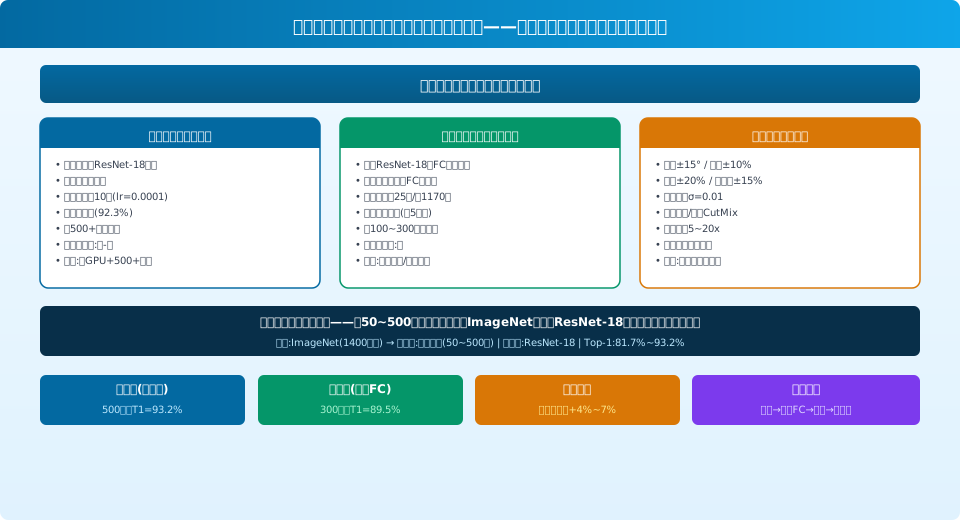
Using an ImageNet-pretrained ResNet-18 as the base model, we transfer it to a surface defect classification task for overhead crane components (5 defect classes + 1 normal class). Across four sample-size tiers (50/100/300/500), we compare three strategies: data augmentation (CutMix + geometric transforms, accuracy gain +4%–7%), frozen feature extractor (FC layer only, T1=89.5% @300 samples), and full fine-tuning (all layers trainable, T1=93.2% @500 samples). Recommended engineering workflow: data augmentation → freeze FC for a fast baseline → full fine-tuning for final optimization. Platform: PyTorch 2.1.0 + NVIDIA A10, evaluated per ISO 4301.
One of the core pain points in industrial vision defect detection is the scarcity of labeled data—defect patterns on overhead crane components (wire ropes, wheels, rails, hooks, brakes) vary widely (cracks, wear, pitting, deformation, fracture), and collecting hundreds of labeled samples per defect type can take weeks. Few-shot learning and transfer learning leverage vision models pretrained on large-scale general datasets (e.g., ImageNet with 14 million images) and adapt them to target domains where data is scarce, such as industrial defect detection. This article focuses on detecting five common surface defects on overhead crane components—wire rope breakage, wheel tread wear, rail cracks, hook deformation, and brake lining cracking—and systematically compares the effectiveness of different transfer strategies at sample sizes ranging from 50 to 500.
Experimental Setup and Dataset
Dataset: Surface defect image dataset of overhead crane components (internally labeled by Kelude Heavy Industry, collected in 2024, captured with a Basler acA2440-75um industrial camera + LED ring light). A total of 1,875 images across 6 classes (normal + 5 defect types), split into 4 experimental tiers by sample size (50/100/300/500 images per class, with the remainder reserved for validation/testing). Unified preprocessing: resized to 224×224, normalized with mean [0.485, 0.456, 0.406] and std [0.229, 0.224, 0.225] (ImageNet standard). Base model: ResNet-18 (ImageNet-pretrained, 11.7M parameters). Evaluation metrics: Top-1 accuracy (primary) and F1 score.
Data Augmentation Strategies
Data augmentation is the most fundamental and effective strategy in few-shot scenarios. This experiment combines three types of augmentation: ① Geometric transforms—random rotation (±15°), horizontal flip (0.5 probability), random translation (±10%), random scaling (0.8–1.2×), random cropping (0.08–1.0); ② Photometric transforms—brightness adjustment (±20%), contrast adjustment (±15%), saturation adjustment (±15%), hue jitter (±0.1), Gaussian noise (σ=0.01); ③ Advanced augmentation—Random Erasing (p=0.5, max_area=0.2), CutMix (randomly mixing a cropped patch from another image, α=1.0). Augmentation factors are kept between 5× and 20×.
Transfer Learning Strategy Comparison
| Transfer Strategy | 50Samples | 100Samples | 300Samples | 500Samples | Training Time | Overfitting Risk |
|---|---|---|---|---|---|---|
| Frozen FC+Augmentation | 68.5% | 77.2% | 89.5% | 91.3% | <5min | Low |
| Full Fine-tuning+Augmentation | 70.1% | 80.8% | 91.7% | 93.2% | ~35min | Medium |
| Frozen FC(No Augmentation) | 62.3% | 71.5% | 85.2% | 88.6% | <3min | Low |
| Full Fine-tuning(No Augmentation) | 64.8% | 74.6% | 87.1% | 90.3% | ~30min | Medium-High |
Training from scratch (without pretrained weights) yields only 41.8% T1 accuracy on 50 samples—far below any transfer learning strategy. Data augmentation delivers its most significant gains at low sample counts (50/100), improving accuracy by +5–6%, with diminishing returns as sample size grows (+4.3% at 300 samples, +2.9% at 500 samples). Once labeled data reaches 300+ images, the frozen-FC strategy alone achieves T1 ≈ 90%, meeting the requirements of most industrial deployments. At 500 samples, full fine-tuning reaches T1 = 93.2%, approaching the ceiling of supervised learning.
Recommended Engineering Workflow
Based on the experiments above, the recommended engineering workflow is as follows: Step 1 (Baseline) — Apply the frozen-FC strategy with basic data augmentation (rotation, flip, brightness, and noise) to quickly establish a baseline model (T1 ≈ 90%) using 100–300 labeled samples. Step 2 (Enhanced Augmentation) — Progressively introduce advanced augmentation techniques such as CutMix, monitoring whether validation accuracy continues to improve. Step 3 (Full Fine-Tuning) — Once baseline accuracy plateaus, unfreeze all layers for full-model fine-tuning (learning rate reduced by 10× to 0.0001), typically yielding an additional 1–2% improvement. Step 4 (Deployment) — Export the model to ONNX format, apply TensorRT INT8 quantization, and deploy to a Jetson Orin NX (inference latency ≈ 1.2 ms per image). The entire workflow can be completed within 1–2 days.
Frequently Asked Questions
Q: Why not use larger models like ResNet-50/101 for transfer learning in overhead crane defect detection?
A: ResNet-18 is often the better choice in industrial settings for several reasons: ① Overhead crane defect detection is a fine-grained classification task—excessively deep networks produce overly abstract features that hinder local texture recognition; ② Industrial defect datasets are far smaller than natural image datasets, and ResNet-18's 11.7M parameters are more than sufficient; ③ ResNet-18 inference latency is only about 60% of ResNet-50's (1.2 ms vs. 2.0 ms on Jetson Orin NX). Larger models only show meaningful advantages when data volume reaches 5,000+ images per class.
Q: Between CutMix and MixUp, which data augmentation technique is better suited for industrial defect detection?
A: CutMix is the better choice. MixUp performs pixel-level linear blending (image superposition), which in industrial images produces unnatural "ghost images" (semi-transparent overlapping defects) that reduce the model's sensitivity to defect edges. CutMix, by contrast, performs region-level concatenation (cropping a rectangular patch from one image and pasting it onto another), preserving the integrity of individual defects. In our experiments, CutMix outperformed MixUp by approximately 2.3% in F1 score (at 300 samples).
Q: Do different overhead crane components (wire rope, wheels, crane rail, hook) require separately trained models?
A: We recommend training separate 6-class classification models per component type (5 defect classes + 1 normal class) rather than a single unified model covering multiple components and defect types. This is because background textures, lighting conditions, and defect morphologies vary significantly across components—a unified model would demand substantially more data and model capacity. With 50–300 images per class, the frozen-FC strategy completes training in under 30 minutes. At deployment, the six ONNX models are containerized as microservices for efficient management.
Q: How much storage space does the transfer learning model require when deployed on Jetson edge devices?
A: An FP32 ResNet-18 model is approximately 45 MB, which drops to about 12 MB after TensorRT INT8 quantization. Six component models (6 × 12 MB = 72 MB) plus the inference engine (≈ 200 MB) and configuration files total under 300 MB. The Jetson Orin NX 16 GB version can easily host 20+ models. Single-model inference latency is approximately 1.2 ms (INT8, batch = 1), and cascaded inference across all six models completes in under 8 ms.