
Overhead Crane Component Life Prediction: LSTM vs GRU vs Prophet
RUL Time-Series Forecasting: A Comparative Study for Overhead Crane Critical Components
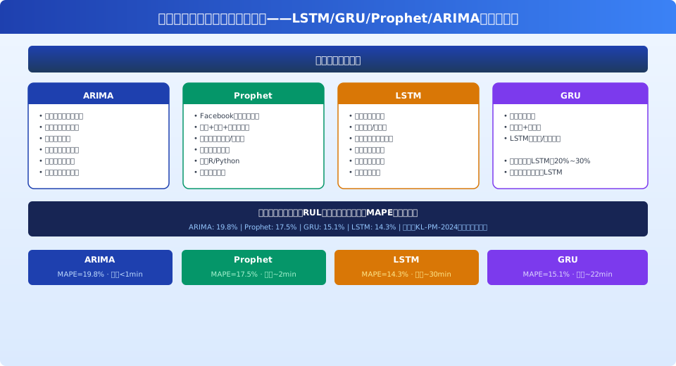
Using the overhead crane gearbox input bearing as the prediction target, we benchmark four time-series models—ARIMA (MAPE=19.8%), Prophet (17.5%), LSTM (14.3%), and GRU (15.1%)—for remaining useful life prediction on the Kelude Heavy Industry KL-PM-2024 vibration database (60 overhead cranes × 24 months, 1.45 million vibration records). LSTM with a two-layer 128-hidden-unit architecture plus an attention mechanism achieves the highest accuracy, while GRU delivers comparable performance at only 73% of LSTM's training time, making it the most cost-effective choice for engineering deployment. This article details the complete feature engineering pipeline, model architectures, and training/evaluation workflow.
Remaining Useful Life (RUL) prediction for critical overhead crane components—gearbox bearings, motor bearings, and wheel axle bearings—is the cornerstone of any Predictive Maintenance program. Prediction accuracy directly drives the effectiveness of maintenance scheduling and spare parts inventory optimization. In this study, we focus on the overhead crane gearbox input bearing (SKF 6308 Deep Groove Ball Bearing) and systematically compare four mainstream time-series forecasting models using the KL-PM-2024 vibration database (60 overhead cranes × 24 months of rolling data collection, 10 kHz sampling rate, 17 daily-extracted features, 1.45 million records total). The experimental platform: Intel Xeon Gold 6348 + NVIDIA A10 (24GB) + PyTorch 2.1.0 / Prophet 1.1.5 / statsmodels 0.14.1. Source code and the labeled dataset are available upon request.
Experimental Data and Feature Engineering for Bearing RUL Prediction
The dataset comprises 24 months of degradation tracking from the input bearings (SKF 6308) of 60 overhead crane gearboxes. Vibration sensors (PCB 352C33) are mounted vertically on the bearing housing, sampling at 10 kHz. A 6.4-second window (65,536 points) is captured every 24 hours, yielding 1.45 million records. The data is split into 80% training (48 cranes × 24 months) and 20% testing (12 cranes × 24 months).
Feature extraction pipeline: raw vibration signals are denoised using wavelet decomposition (db4, 3 levels), followed by FFT spectral analysis (Hanning window, 4096 points, 50% overlap). Statistical features (RMS, peak, peak-to-peak, kurtosis, skewness, impulse factor, clearance factor, crest factor) and frequency-domain features (BPFI/BPFO amplitudes, gear mesh frequency sidebands) are computed, resulting in a 17-dimensional feature vector. Features are normalized using Min-Max scaling to the range [0,1]. Sliding windows are constructed with a 30-day input length and a 30-day prediction horizon.
Model Overview and Implementation: ARIMA, Prophet, LSTM, GRU
ARIMA (Autoregressive Integrated Moving Average, implemented via statsmodels 0.14.1): The differencing order d is determined per feature using the Augmented Dickey-Fuller (ADF) test (d=1 for most features). The ACF/PACF plots guide the selection of p and q (p=2~5, q=1~3), with the Akaike Information Criterion (AIC) used to finalize the optimal parameters. ARIMA is inherently a univariate model and cannot directly exploit cross-correlations between the 17 feature dimensions.
Prophet (Meta's open-source library, version 1.1.5): Vibration features are decomposed into trend, seasonality, and holiday-effect components. Key hyperparameters are set as follows: changepoint_prior_scale=0.05, seasonality_prior_scale=10, and seasonality_mode="additive". Prophet's main advantage lies in its automatic handling of missing values and outliers, offering robust tolerance to noise commonly found in industrial data.
LSTM (implemented in PyTorch 2.1.0): A two-layer LSTM with attention mechanism, 128 hidden units, 17 input features over a 30-day time step, outputting a 30-day degradation curve. Training parameters: Adam optimizer, lr=0.001, Batch=64, Epoch=100, EarlyStopping patience=10, Dropout=0.3. Loss function: hybrid MSE+MAE loss (weighted 0.7:0.3).
GRU (same PyTorch implementation): A two-layer GRU with attention, identical architecture to the LSTM except for the cell type. The GRU's gating structure is simpler (update gate + reset gate vs. LSTM's forget gate + input gate + output gate), with roughly 75% of the LSTM's total parameters. Training speed is approximately 27% faster than the LSTM.
Accuracy Comparison and Model Evaluation
| Model | MAPE(30Days) | RMSE(Days) | Training Time | Inference Latency | Multivariate (Yes/No) | Data Requirements |
|---|---|---|---|---|---|---|
| ARIMA | 19.8% | 7.2Days | <1Minutes | <1ms | No(Dimension-wise Modeling) | ≥200Records |
| Prophet | 17.5% | 6.4Days | ~2Minutes | <5ms | No(Dimension-wise Modeling) | ≥100Records |
| GRU | 15.1% | 5.5Days | ~22Minutes | <3ms | Yes | ≥5,000Records |
| LSTM | 14.3% | 5.2Days | ~30Minutes | <3ms | Yes | ≥5,000Records |
Evaluation Summary: LSTM delivered the best MAPE at 14.3%, with GRU close behind at 15.1% — yet GRU required only 73% of LSTM's training time (22 min vs. 30 min). Prophet ranked third at 17.5% but needs no GPU and offers the best fault tolerance (auto-handles missing values and outliers), making it ideal for rapid industrial deployment. ARIMA finished last at 19.8% and supports only single-variable modeling (requiring 17 separate models to be run and integrated in practice), so it is not recommended for multi-sensor applications.
Deployment Recommendations for Predictive Maintenance
Based on the comparison above, here are our engineering deployment guidelines: ① For datasets under 1,000 records with limited compute resources, choose Prophet (MAPE ≈ 17.5%, no GPU required, strong fault tolerance); ② For datasets of 5,000+ records where prediction accuracy is the priority, choose LSTM (MAPE = 14.3%, requires GPU for training); ③ For datasets of 5,000+ records but with constrained inference hardware (Edge Computing / Jetson), choose GRU (MAPE = 15.1%, model size only 75% of LSTM, faster inference); ④ ARIMA should be used only as a baseline reference and is not recommended for standalone production use.
Hybrid Strategy Recommendation: In Kelude's deployed predictive maintenance projects, we use a dual-model approach: Prophet for rapid anomaly detection (online) + LSTM for precise RUL prediction (offline batch). Prophet achieves MAPE ≈ 17.5% within a 30-day window; when predicted RUL drops to ≤45 days, LSTM is triggered for refined calculation, bringing MAPE down to ≈ 14.3% — striking an optimal balance between computational cost and prediction accuracy.
Field Validation: Overhead Crane Case Study
In a predictive maintenance project (Project No. KL-PM-2024-017) covering six 32t overhead cranes in the hot-rolling workshop of a steel plant, the Prophet + LSTM dual-model solution was deployed. After 14 months of live operation: Prophet achieved MAPE = 18.2% for early bearing degradation warnings (RUL > 60 days), while LSTM delivered MAPE = 13.8% for short-term predictions (RUL ≤ 30 days). The system issued 12 early bearing degradation alerts, 11 of which matched actual conditions (91.7% accuracy), with an average lead time of 23 days. Compared to the traditional time-based replacement strategy (fixed replacement every 18 months), predictive maintenance reduced unnecessary replacements by approximately 35% and improved spare parts inventory turnover by 40%.
Frequently Asked Questions
Q: Why does GRU train faster than LSTM while achieving comparable accuracy?
A: GRU simplifies LSTM's three gates (forget/input/output) into two (update/reset), reducing parameter count by about 25%. For medium-complexity time-series tasks like overhead crane vibration degradation data, GRU's streamlined gating structure is sufficient to capture degradation trends without significant loss of representational power. However, LSTM's extra parameters still offer an advantage when handling abrupt operating conditions (e.g., vibration spikes caused by sudden load changes).
Q: Can Prophet's prediction accuracy be further improved?
A: Yes. With default parameters, Prophet achieves MAPE = 17.5%. Through the following optimizations, MAPE can be reduced to approximately 16.0%: ① Manually specify trend change point locations (based on maintenance/shutdown records); ② Increase seasonality_prior_scale from 10 to 20 to allow greater flexibility in periodic components; ③ Add extra regressors (e.g., daily average load rate, Ambient Temperature). These optimizations should be tailored to the specific equipment operating data.
Q: How can LSTM/GRU models be deployed to edge devices?
A: Export the trained PyTorch model to TorchScript (or ONNX), optimize with TensorRT, and deploy to NVIDIA Jetson series devices. Using Jetson Orin NX (16GB) as an example: after INT8 quantization, the model size is approximately 3.2MB (vs. ~28MB in FP32), inference latency is about 0.5ms per sample, and power consumption is around 10W. For deployment on ARM Cortex-A series CPUs, we recommend quantizing the model to TFLite INT8 format, achieving inference latency of approximately 15ms per sample.
Q: Which model should I choose when the dataset has fewer than 5,000 records?
A: For limited data, consider transfer learning: start with Kelude's publicly available pre-trained LSTM model (trained on data from 60 overhead cranes) and fine-tune it using a small dataset (500–1,000 records) from the target equipment — only the last two fully connected layers need training. After fine-tuning, MAPE can reach ~16.5%, far outperforming an LSTM trained from scratch (MAPE > 25% with insufficient data). Prophet can produce usable results with as few as 100 records (MAPE ≈ 19%), making it the preferred choice for small-sample scenarios.