

Knowledge Distillation: Shrink AI Model Size Without Losing Accuracy
📋 Key Summary
Knowledge distillation is, at its core, a process where a fully trained large model (the teacher) transfers its output probability distribution—the soft labels that capture inter-class similarities—to a much smaller model (the student). Instead of memorizing hard labels, the student learns from the teacher's soft labels, allowing it to retain most of its accuracy while compressing the parameter count by roughly an order of magnitude. This article covers the four boundary conditions for distillation, the loss derivation for temperature softening and KL divergence, a worked verification example for crane defect detection, and four common mistakes. Applicable operating conditions: the teacher model is already running on a server with acceptable accuracy, and the goal is to shift inference to edge devices for real-time response and low power consumption. Not applicable: when teacher accuracy is insufficient, when training and deployment data distributions diverge significantly, or when strictly interpretable decision-making is required.
Let's run the numbers: when deploying visual inspection models on edge devices for cranes, accuracy and model size are fundamentally at odds. A deep model with dozens of layers can easily carry hundreds of millions of parameters—it detects wire rope broken wires and judges load position more reliably, but it either runs on a server with inference latency in the tens of milliseconds, or it simply overwhelms an edge box. For pick-and-place alignment and online inspection that demand millisecond-level response, tens of milliseconds of latency is already a liability.
On the flip side, a purely small model delivers low latency and low power consumption—a few watts on an edge box—but accuracy often falls short. When you add it all up, the cloud-side large model has ample computing power but high latency, while the edge-side small model has low latency but weaker accuracy. The accuracy gap in between is exactly what knowledge distillation is designed to fill—not by upgrading hardware, but by having the large model teach the small model how to make judgments.
It sounds like "passing the craft from master to apprentice," but in engineering, it comes with a computable loss function and boundary conditions. Kelude has repeatedly validated one thing in edge inference deployment: whether distillation succeeds depends first on getting the boundary conditions right, not on how fluently you can recite the formulas. Let's start with those boundary conditions and work through the math.
When Is Knowledge Distillation Worth It? Four Boundary Conditions
The first boundary condition: the teacher model must already meet acceptance criteria. Knowledge distillation is knowledge transfer, not model repair. If the teacher's own accuracy fails to pass muster, distillation will simply pass its learned mistakes on to the student—and because the student has less capacity, those errors get amplified. Kelude's principle for edge deployment is straightforward: train the large model on a server until it satisfies acceptance criteria, then talk about compression.
The second boundary condition: the deployment target must be clearly defined. If the final destination is an edge box with millisecond-level latency requirements and only a few watts of power, then compressing the large model delivers clear benefits. If the model runs on a server cluster where latency is not a concern, distillation lacks a driving incentive. The computing power budget sets the ceiling for the student model—and determines whether the whole exercise is worth doing.
The third boundary condition: the training data and deployment data must share the same distribution. A distilled student model has less capacity and weaker generalization, making it more sensitive to data drift. The larger the gap between the training set and the actual operating conditions, the more the student's accuracy loss is magnified. The fourth boundary condition: the acceptable accuracy loss must be quantified upfront—distillation almost always introduces some accuracy drop, and the key question is whether that drop stays within the project's allowable range, as verified under real operating conditions.
| Parameter | Definition | Typical Value | Impact ondistillationInfluence |
|---|---|---|---|
| Teachermodel parameter count | Cloud LLM Scale | Hundreds of Millions(Project-Specific) | Larger Leads to OverfittingParameterCompression,Higher Compressibility |
| Studentmodel parameter count | Edge Model Scale | Millions | Determines Edgelatencyandpower consumption |
| TemperatureCoefficient T | SofteningsoftmaxScale | 4~8(Task-Specific Tuning Required) | Higher Temperature Softer Distribution、More Dark Knowledge |
| Loss Weight α | Soft-to-Hard Loss Ratio | 0.5~0.9 | Balances Inter-Class Relations and Ground Truth |
| training dataVolume | Labeled Sample Size | andTeachertraining setSame Distribution | Data Drift Amplifiesaccuracy loss |
| inference latencyObjective | Edge Single Inferenceinference time | Millisecond-Level(Based onoperating conditionProject-Specific) | Determines Studentmodel sizeUpper Bound |
| computing powerandpower consumptionBudget | Edge Available Resources | Several Watts~Tens of Watts | Determines Student Deployability |
| AccuracyRetention Target | Acceptable Degradation vs. Teacher | Based on Actualoperating conditionAcceptanceProject-Specific | DeterminesdistillationFeasibility Decision |
How Is Distillation Loss Calculated? Deriving Temperature Softening and KL Divergence
At the heart of knowledge distillation is a single goal: making the student model's output distribution match the teacher model's as closely as possible. Two mechanisms drive this process—temperature softening and KL divergence.
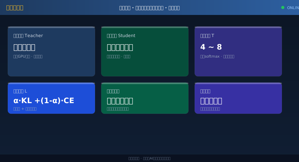
The first step is temperature softening. A standard softmax maps logits to a hard, near-one-hot probability distribution, but distillation first divides the logits by a temperature coefficient T to flatten the distribution. The higher the temperature, the smoother the distribution becomes, and the relative differences between classes emerge more clearly. The softened probability is expressed as:
q_i = exp(z_i / T) / Σ_j exp(z_j / T)
Here, z_i is the raw logit output of the model for class i, T is the temperature coefficient, and q_i is the softened probability.
The second step measures the divergence between the student and teacher distributions. The loss function uses KL divergence (relative entropy) to quantify how dissimilar the two probability distributions are. The softened distillation loss is written as T² multiplied by the KL divergence—the T² factor compensates for the gradient scaling introduced by temperature. The final total loss is a weighted combination of the softened and hard losses:
L = α · T² · KL(q_teacher ‖ q_student) + (1 − α) · CE(y_true, p_student)
Where α is the weight assigned to the softened loss, CE is the cross-entropy loss against the ground-truth labels, and p_student is the student model's standard output at temperature T = 1.
Why keep the hard-label term at all? Because soft labels teach the relationships between classes, while hard labels ensure the student never drifts too far from the correct answer. Both are indispensable. The weight α typically falls between 0.5 and 0.9, with the exact value determined through hyperparameter tuning.
A Worked Verification Example: Compressing a Crane Defect Detection Model from Hundreds of Millions to Millions of Parameters
Let's tie the formulas above to a concrete scenario. Suppose a facility needs online inspection of surface defects on wire ropes. The teacher model is a large network trained on a server, with a parameter count in the hundreds of millions. Its training data comes from a defect image library accumulated over years of on-site operation—datasets of this kind typically range from tens of thousands to hundreds of thousands of images in the industry, and Kelude's defect annotation system continues to grow such samples. Once the teacher model meets accuracy targets on the server, it is distilled into a student model with only a few million parameters, deployed to an edge computing box that performs frame-by-frame detection on wire ropes in service.
The core question in this verification exercise is straightforward: after all that compression, is the accuracy still acceptable? There is no one-size-fits-all answer—the relative accuracy loss after distillation depends on a chain of variables, including the teacher model's redundancy, the temperature T, and the volume of training data. The only reliable way to know is to test under actual operating conditions. That said, one engineering pattern holds fairly consistently: the larger and more over-parameterized the teacher model, the greater the compressibility, and the higher the proportion of accuracy that distillation can preserve.
| Indicator | Teacher Model | Student Model(distillationPost-) | Remarks |
|---|---|---|---|
| parameter count | Hundreds of Millions | Millions | Compression by ~1 Order of Magnitude |
| Edge Single Inferenceinference latency | serverTens of Milliseconds | Edge Millisecond-Level | Based on Actualoperating conditionMeasured Values Prevail |
| Deployment Location | Cloud/server | Edge Box/Embedded | Data Notfactory、Faster Response |
| Relative toAccuracy | Baseline(Denoted as100%) | Retains Majority | Actual Degradation Measured |
| power consumption | serverHundreds of Millions | Several Watts~10-20 Watts | Edge Lowpower consumptionOperation |
From the results, the student model compresses the parameter count by roughly an order of magnitude, cutting inference latency from tens of milliseconds at the server level to single-digit milliseconds at the edge, while power consumption drops to a range of a few watts to around fifteen watts. These gains translate directly into real-time-sensitive operations such as grab positioning and online inspection. In Kelude's edge deployment approach, these distilled compact models serve as the primary inference units, while the large model remains on the training side or acts as a fallback for manual review.
One boundary condition needs to be made explicit: the output of these edge-side inspection models must ultimately feed into the crane's safety monitoring and interlock logic. The deployment boundary must satisfy the data acquisition and real-time requirements defined in GB/T 28264 Safety Monitoring and Management System for Lifting Appliances, while load and operating-condition judgments involving the model still need to operate within the framework defined by FEM 1.001 Crane Design Standard. Knowledge distillation does not alter these safety boundaries — it only changes the model's size and speed.
Four Common Mistakes That Waste Your Distillation Effort
Mistake one: rushing to distill before the teacher model is properly trained. Garbage in, garbage out — distillation amplifies the teacher's existing deviations rather than compensating for them.
Mistake two: setting the temperature T incorrectly. If T is too low, soft labels degrade into hard labels and the dark knowledge is lost; if T is too high, the distribution becomes overly smooth and the student fails to learn discriminative power. The temperature needs to be tuned per task — there is no one-size-fits-all value.
Mistake three: learning only soft labels and discarding hard labels. Soft labels teach relationships, hard labels guarantee correctness — both are indispensable, and the loss weight α is there to balance them.
Mistake four: ignoring data distribution drift. A student model has smaller capacity and weaker generalization; once training data and deployment operating conditions fall out of alignment, accuracy loss gets amplified. Distribution verification is required both before and after distillation.
Compressing a large model's accuracy into a small model is, at its core, a computable trade-off among three variables: accuracy, latency, and power consumption. In Kelude's edge AI deployment, knowledge distillation serves as one of the means to push heavyweight model capabilities down to edge boxes, combined with upstream steps such as data cleaning and semi-supervised learning — so that cranes can perform detection and early warning close to the worksite instead of waiting on the cloud for everything. The premise remains unchanged: boundary conditions must be worked out first, and accuracy loss is accepted only through measured verification.
📖 Related reading: Running AI Models on Crane Edge Devices: How to Balance Accuracy Against Compute Cost | What Large Models Can Actually Deliver in Crane Maintenance Operations
FAQ
Q: After distillation, does the compact model deployed at the edge still meet the real-time requirements of crane safety monitoring?
A: Knowledge distillation changes the model's size and inference speed, not the system's safety function boundaries. Using the data acquisition and real-time requirements of GB/T 28264 Safety Monitoring and Management System for Lifting Appliances as the reference, deployment is acceptable as long as the distilled model's inference latency and accuracy meet the engineering acceptance criteria, and the model output still feeds into the existing interlock and manual review processes. Kelude has always held this line in its edge solutions: specific indicators must be verified item by item against actual operating conditions during project acceptance — a smaller model is never a reason to skip safety verification.
Q: When is knowledge distillation not worth doing, and how do you decide whether a project should go down this path?
A: Watch for three signals. First, if the teacher model's own accuracy falls short, distillation will pass those errors straight down to the student. Second, if there is a significant gap between training data and deployment operating conditions, the student's weaker generalization makes drift more pronounced. Third, if the edge computing budget can already run the large model comfortably, the compute-saving argument loses its basis. If any one of these three signals appears, fix the data and teacher-model issues first — then talk about distillation.
Q: Why does a small model learn more accurately from a large model's soft labels than from hard labels directly?
A: Because the teacher model's softmax output doesn't just say which answer is correct — it also reveals how similar each answer is to the others, and that probability distribution is the dark knowledge. For example, given a wear image, the teacher might output wear 0.7, corrosion 0.2, normal 0.1. When the student learns this distribution, it also picks up the relationship that wear and corrosion are feature-adjacent. That carries far more information than memorizing a single hard label — and that is the fundamental reason distillation preserves accuracy.
