

LSTM vs Transformer for Crane Time Series Forecasting: How to Choose
📋 Key Summary
Time-series forecasting is the backbone of predictive maintenance for cranes: it enables models to capture degradation trends from historical sequences of vibration, current, and temperature data, providing an early warning window before failures occur. This article focuses on the two mainstream approaches—LSTM and Transformer. We first define the boundary conditions for input sequences, then walk through the core formulas behind each method, and close with a worked verification example on a vibration sequence, offering a selection framework based on computational complexity and deployment cost. It should be noted that the effectiveness of time-series forecasting is highly dependent on operating conditions and data quality; we do not promise a universal accuracy figure, but rather a practical decision-making framework.
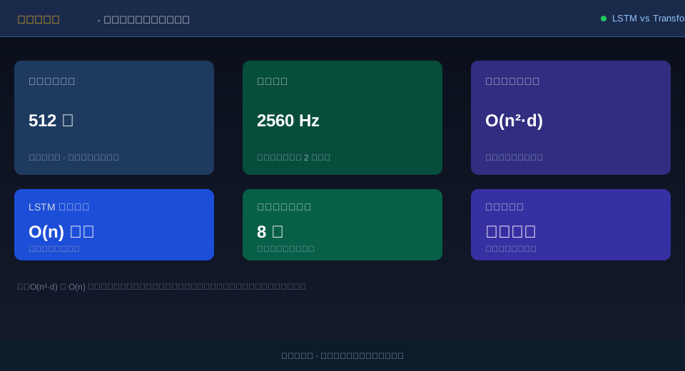
Defining Input and Output Boundaries for Time-Series Forecasting: Sequence Length, Sampling Rate, and Data Volume
Let's start with the bottom line: time-series forecasting is not about dumping all historical data into a model and expecting results. The model takes multi-channel sequences arranged in chronological order as input and outputs predicted values or health indicators for future steps. Whether the boundary conditions are set correctly determines if the model learns real degradation patterns or just sampling noise.
From a data source perspective, parameter acquisition for lifting appliances is not designed in a vacuum. GB/T 28264 Safety Monitoring and Management System sets unified requirements for the types of monitored parameters, data acquisition, and recording in safety monitoring and management systems. Key quantities such as lifting capacity, travel speed, and lifting height all have clear acquisition specifications. When Kelude deploys condition monitoring, these specifications typically serve as the baseline for data acquisition, with high-frequency signals like vibration and current added as input channels for time-series forecasting.
Sampling frequency is the second boundary. Take gearbox vibration as an example: gear meshing frequencies typically fall in the hundreds of hertz range, so the sampling frequency must be at least twice the highest fault characteristic frequency. Otherwise, aliasing occurs—high-frequency fault features fold into lower frequency bands, and the model ends up looking at a contaminated spectrum. Sequence length, on the other hand, determines how much historical context the model can see. Too short, and it misses complete rotation cycles; too long, and it drags in irrelevant history that adds noise.
Data volume is the third boundary. The training set must cover combinations of different lifting capacities, load rates, and rotational speeds; otherwise, the model fails as soon as the operating condition changes. The work duty of cranes is classified from A1 to A8 in FEM 1.001 Crane Design Standard, with each level corresponding to a distinctly different load spectrum. A model trained only on A3 light-duty conditions will inevitably produce inaccurate predictions when applied to A6 heavy-duty conditions. This point is often underestimated, yet it is the most direct reason why time-series models degrade after deployment.
LSTM Gating vs. Transformer Self-Attention: A Formula-Level Breakdown of What Each One Computes
To decide which one to use, you first need to understand what each does mathematically. The core of LSTM is its gating mechanism—three gates control what information to keep and what to forget. The core of Transformer is self-attention, which lets every position in the sequence directly connect with every other position.
In one time step of LSTM, the previous hidden state and the current input are concatenated and passed through learnable weight matrices to compute three gates and a candidate memory:
Forget gate: f_t = σ(W_f·[h_{t-1}, x_t] + b_f)
Input gate: i_t = σ(W_i·[h_{t-1}, x_t] + b_i)
Candidate memory: c~t = tanh(W_c·[h_{t-1}, x_t] + b_c)
Cell state: c_t = f_t ⊙ c_{t-1} + i_t ⊙ c~t
Output gate: o_t = σ(W_o·[h_{t-1}, x_t] + b_o)
Hidden state: h_t = o_t ⊙ tanh(c_t)
The three gates are essentially a set of sigmoid outputs, with values between 0 and 1, applied element-wise to the state vector to achieve weighted retention of information. The cell state c_t acts as the main highway running through the entire sequence—gating only performs linear additions, so gradients can propagate relatively stably along this path, mitigating the vanishing gradient problem in long sequences.
Transformer takes a different route: instead of relying on sequential propagation, self-attention computes a similarity score between every position and every other position, then aggregates values weighted by those similarities. The attention scoring formula is:
Attention scoring: Attention(Q, K, V) = softmax(QK^T / √d_k) · V
Here, Q, K, and V are the query, key, and value matrices, respectively. Dividing by √d_k prevents the dot product from becoming too large and pushing softmax into its saturation region. Multi-head attention splits Q, K, and V into multiple subspaces computed in parallel, allowing the model to capture dependencies at different scales simultaneously. When this formula lands in Kelude's engineering practice, the real challenge is never the formula itself—it's how to set the hyperparameters in the table below.
| Symbol | Name | Typical Value/Meaning | Engineering Note |
|---|---|---|---|
| n | Sequence Length | Input Window Sample Count,e.g.512 | Larger receptive field,computing powerHigher computational cost |
| f_s | sampling frequency | e.g.2560 Hz | Must exceed maximum faultcharacteristic frequency2times or more |
| d | Feature Dimension | Per Time Stepaccess systemInput Window Sample Count | vibration、Current、Temperature, etc.access systemConcatenation |
| h | Number of Attention Heads | Commonly Used8 | More headsParameterMore heads,Requires matching data volume |
| d_k | Head Dimension | Equalsd/h | softmaxPre-scaling Factor |
| σ | sigmoidActivation | Output Range(0,1) | Gating Retention Ratio |
| tanh | Hyperbolic Tangent (tanh) | Output Range(-1,1) | Candidate Memory Nonlinearity |
| ⊙ | Element-wise Multiplication | Gate-state Multiplication | Selective Memory Implementation |
Sequence Length in Vibration Analysis: Does a Longer Sequence Always Mean a Better Model?
Let's tie the parameters above together with a worked example. Assume a crane gearbox input shaft running at 1000 r/min, a driving wheel with 21 teeth on the primary gear pair, and a vibration sensor sampling at 2560 Hz. The following calculations are for demonstrating the quantitative relationships between parameters only—actual values depend on site-specific operating conditions.
First, the rotational frequency: dividing the input shaft speed of 1000 r/min by 60 gives a rotational frequency of approximately 16.7 Hz. Next, the gear mesh frequency: multiplying the tooth count of 21 by the rotational frequency yields roughly 350 Hz. The Nyquist frequency corresponding to a 2560 Hz sampling rate is 1280 Hz, which covers the 350 Hz fundamental frequency and its third harmonic at 1050 Hz—this sampling configuration is reasonable from an engineering standpoint.
Now consider sequence length. The number of samples per rotational period is 2560 divided by 16.7, or about 153 points. With a sequence length of 512 points, the window spans roughly 3.3 rotational periods, which is sufficient to capture the vibration waveform across several complete rotation cycles of the gear pair. Stretching the sequence to 4096 points extends coverage to about 26.7 periods—a much larger receptive field—but the self-attention computational cost jumps from 512² to 4096², an increase of roughly 64 times.
This is the mathematical reason why a longer sequence is not always better: receptive field grows linearly, while self-attention computation grows quadratically. In Kelude's selection process, the typical approach is to first compress the sequence length to cover several complete fault cycles, then gradually extend it for comparison testing.
| Item | Formula | Result | Description |
|---|---|---|---|
| Rotational Frequency f_r | 1000 / 60 | 16.7 Hz | Input ShaftRotational speedConverted |
| MeshingFrequency f_m | 21 × 16.7 | Approx.350 Hz | First StageGearSecondary |
| Samples per Cycle | 2560 / 16.7 | Approx.153Points | One Rotational Frequency Cycle |
| 512PointscoverageOne Rotational Frequency Cycle | 512 / 153 | Approx.3.3Units | Input Window |
| NoteTorqueMatrix Size | 512 × 512 | 262144Pair | Quadratic Cost |
Four Most Common Time-Series Forecasting Pitfalls: Data Leakage, Sequence Length, Overfitting, and Label Misalignment
When a time-series model degrades after deployment, the root cause is often not an outdated model architecture but flaws in the data engineering pipeline. The four categories of errors below are ranked by severity, from highest to lowest impact.
Error #1: Data Leakage. This occurs when future information leaks into the training features—for instance, normalizing with statistics derived from the entire dataset or applying test-set statistics to the training set. The model performs exceptionally well on the validation set but collapses immediately upon deployment. Time-series data must be strictly split chronologically, with no overlap between the training, validation, and test sets.
Error #2: Mismatch Between Sequence Length and Sampling Rate. A sampling rate that is too low causes high-frequency fault characteristics to alias, producing a distorted frequency spectrum for the model to learn from. Conversely, a sequence that is too short may not even capture a single complete rotation cycle. The correct approach is to first calculate the rotational frequency and meshing frequency, then work backward to determine the appropriate sampling rate and sequence length.
Error #3: Model Overfitting. Transformers have a large parameter count and are highly prone to overfitting when training data is insufficient. You might see the training loss steadily decrease while the validation loss climbs higher. In this situation, the priority should be to reduce model size and increase regularization, rather than continuing to add more data or scaling up the model.
Error #4: Label Misalignment. This happens when sensor readings at time t are paired with fault labels from time t+1, or when the alarm timestamp is mistakenly treated as the fault onset time. A single sampling point of label shift causes the entire prediction target to drift. At Kelude, we always perform a time-alignment review on labels during the annotation of time-series data—this is the most easily overlooked yet most critical step in the entire pipeline.
Returning to the question posed in the title: LSTM or Transformer? In scenarios like crane condition monitoring, where data volume is limited and sequences are relatively short, LSTM is typically the more robust starting point. It has a smaller parameter count, trains more stably, and has lower deployment costs on edge devices. Only when the data accumulates to a sufficient scale and global, long-range dependencies need to be captured should you consider introducing a Transformer or using it for multi-channel fusion. There is no one-size-fits-all answer to model selection—only the answer that fits your specific operating condition. Define the boundary conditions first, then calculate the computational complexity, and finally validate with small-scale experiments. This is the deployment sequence Kelude has repeatedly verified in practice.
📖 Related Reading: Equipment Health Management (PHM): An Engineering Practice of Big Data and ML-Driven Predictive Maintenance for Overhead Cranes | What Can Large Models Actually Do for Crane Maintenance? Practical Scenarios and Capability Boundaries
FAQ
Q: What are the requirements for monitoring operating parameters under the safety monitoring system for lifting appliances?
A: The GB/T 28264 standard for Safety Monitoring and Management Systems requires real-time monitoring and recording of key operating status parameters such as Lifting Capacity, Travel Speed, and Lifting Height. This provides a unified data foundation for subsequent fault analysis and time-series prediction. When Kelude builds a condition monitoring platform, we first categorize the data acquisition points according to the parameter classifications in this standard, then layer on high-frequency signals like vibration and current. The specific parameters and recording intervals should be determined based on the current version of the standard and on-site inspection requirements.
Q: What level of prediction error is considered acceptable for a time-series model to be deemed usable?
A: Whether the prediction error is acceptable depends on the trade-off between early warning lead time and the false alarm rate; there is no universally applicable threshold. The key criteria are whether the early warning provides a sufficient maintenance window and whether the frequency of false alarms remains within a tolerable range for maintenance personnel. Baselines vary significantly across different crane models and operating conditions. Specific thresholds should be established through on-site validation, with the actual operating condition serving as the final reference.
Q: Why is LSTM often the first choice in industrial settings, even though Transformers are theoretically more powerful?
A: Because industrial time-series data is often limited in volume and sequence length. The self-attention mechanism in Transformers requires substantial data to leverage its global modeling advantage; with insufficient data, it is prone to overfitting. LSTM, with its simpler structure and smaller parameter count, is more stable on small-sample sequences. Additionally, the quadratic complexity of Transformers creates significant computing power demands when deployed on edge devices. For these reasons, Kelude typically uses LSTM as the baseline model and decides whether to introduce a Transformer based on the scale of available data.
